Weir PW
Mapping Dose, Exposure Latitude, Focus and Depth-of-Focus Uniformity
for Improved Process Setup and Characterization
See Also:
Weir PW Brochure,
ML06 Bossung Focus
Related Tutorials: Focus and Depth-of-Focus Uniformity
Applications: Process comparison, Process setup, control, yield enhancement,
reticle qualification, OPC characterization, dose mapping,
improved process window selection.
User's Area - Requires Logon:
Other tutorials in the user's section: White Paper Tutorials
Contact TEA Systems for a Weir Demonstration or Logon
Minimizing across chip linewidth variation (ACLV) is critical for both process stability and yield. Therefore if features respond differently during imaging then their process window response will also vary depending on the characteristics and imaging neighborhood of the feature.
Process setup and yield performance are optimized when the influence of the individual exposure tool is removed during characterization. The technique described in this section provides full-profile and full-field mapping of Exposure-Dose uniformity needed for a reticle to function within and be centered upon the process window. The results can then be used to enhance yields by biasing the dose during exposure and by validation of each critical feature site after reticle manufacture.
Exposure Latitude (EL%), Depth-of-Focus (DoF) and Best Focus uniformity are also sensitive to the mask structures and process operating point. This method can be equally well applied to these metrics to optimize production yields.
Questions addressed by this technique
-
How sensitive are process-windows settings to site and feature selection?
-
How can the effective exposure-dose be influenced by the reticle-scan?
-
What is the variation in dose from feature-site to site?
-
What components of the CD-variation are contributed by the process or exposure tool?
-
How can the influence of the exposure tool be removed in process and film evaluations?
-
How can we clearly see performance differences between multiple Anti-Reflective Coatings or film thickness?
-
What portion of the across-chip-linewidth-variations (ACLV) is contributed by the exposure-tool, reticle and process?
-
How does the effective Exposure-Latitude (EL%) vary across the field?
-
How can we insure that a new reticle behaves uniformly to exposure-dose?
-
What are the optimized OPC structures for my combination of process and exposure-cell* setup?
Keywords: Mapping, Dose, Exposure-Dose, Exposure, Contour, Process Setup, Control, OPC, Site Uniformity, Metrology, Process window, full field, full profile, Yield Enhancement, Feature Response, Optimum Focus Response
Objectives
- The advantages of deriving dose from multiple product features rather than a single point in the exposure.
- Data import and setup using Weir PW
- One site performance comparison to full-field response
- Dose-setting using an analysis of the full-field uniformity instead of a statistical average.
- Converting feature information to Dose and Exposure-latitude uniformity across the field
- Enhanced process window designation
- Derived feature uniformity without exposure-tool perturbations.
- Final Reticle and OPC design qualification and validation.
- Reticle process characterization and uniformity
Table of Contents
Removing Exposure-Tool Influence: True Process Response to Dose
Dose @ Best Focus Reports & Graphs (True Process Response)
Introduction
If you work with feature sizes that extend below the 90 nanometer (nm) node then you've experienced the frustration of setting up the process window only to find feature uniformity can quickly vary out of control during production in very unexpected ways. With the risk of repeating an overused cliché in our industry, as feature sizes continue to shrink, so do the process margins and our ability to live within them.
It's a well known
fact that feature size, profile response and edge roughness vary with focus and
the exposure-dose. Consideration must extend beyond this simple concept to
maintain a stable sub-90 nm process. Typically the strongest contributor to ACLV
is the feature's as-manufactured structure on the reticle. Reticle enhancement
techniques (RET) such as optical proximity correction (OPC) and phase-shifting (PSM)
further complicate these variations because the combined process variations of
photomask manufacturing is convoluted against the perturbations of the
lithography-cell* exposure sequence. This convolution can result in feature
response that will vary across the exposure field in a manner that cannot be
anticipated by any current simulation technique.
Exposure tool vendors have announced the ability to bias exposure-dose during the reticle scan thereby improving ACLV. However, the methods for calculating dose-uniformity on a site-by-site basis are not shown nor is a consideration for whether the variation is due to the exposure cell or reticle.
Weir PW provides the tools needed to map exposure dose uniformity and the method as shown below is quite simple. During this mapping you will enjoy the added benefit of easily mapping full process-window uniformity across the field of exposure including the metrics of exposure latitude, focus and depth-of-focus.
Process Response Surface
The interpretive curve of feature size as a function of focus error was first described by John Bossung in 19771 and a typical feature-response to dose graph is shown for two sites on the field in figure 1. The upper and lower control limit (UCL and LCL) lines delineate the acceptable response limits of the feature. The feature for site "A" will generate acceptable characteristics for any dose (abscissa) values that reside within the two control limits. The Exposure Latitude (EL) is defined as the range of dose values in this region. The exposure latitude is typically presented as a percentage of the average dose values for this range or:
EL% = (Dmaximum - Dminimum) / Dmean * 100)% (1)
If we next plot the dose-response for a second feature on the reticle the new curve will rarely overlay the first curve. A typical response curve for a second reticle site is shown by curve "B" in figure 1. The variation in response can be caused by a number of factors including feature design for proximity, reticle manufacturing, changes in reticle-scan stage speed, localized exposure-dose and effective coherence and numeric aperture of the lens and wavefront focus errors.
A constant offset between the two curves results from simple design or reticle manufacture and these variations are predicable by simulation methods. Curves that vary in slope and curvature result from the complex interactions of the reticle feature with the perturbations of the exposure conditions and even the film stack for base, photoresist and anti-reflective coatings (ARC). A major contributor to the curvature of the response is the localized focus error resulting from lens aberrations, illumination settings and the reticle-scan as shown in the process-window control surface of equation #2.
![]()
where anm is the process coefficient, "F" is the focus and "E" is the exposure-dose2,3.
Since each feature's size will vary in response from it's neighbors, the "best dose" for the process is the exposure at which the exposure latitude is maximized for all critical feature sites on the reticle. In our example shown in figure 1 the best dose will occur at the "Do" exposure shown.
Significant variation between curves will result if there is a problem with the reticle feature design or it's manufacture. This analysis is therefore a good tool for evaluation of new reticles and re-qualification of existing in-use masks for process degradation. Alternatively if the features vary systematically across the exposure field, the fault can be the result of the reticle manufacturing process or the electro-optical system of the exposure tool.
To properly
determine the process setup point, a family of dose-curves is taken for each
focus-offset of the exposure tool. Each "focus-family" will exhibit a best-dose
and exposure latitude. For any dose, the subset of exposure-tool focus curves
that lie within the control limits will represent the depth-of-focus for the
dose and site. The optimum dose will therefore be that at which the exposure
latitude and the associated depth-of-focus (DoF) are maximized.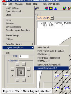
Exposure-cell Specific and Generalized Process Setup
Process windows are simulated for the general process description using algorithms similar to equation #2. These approaches do not incorporate the local response variations of the exposure cell and process films nor do they consider the variations of the photomask manufacture.
If the objective is to evaluate a new photoresist, ARC or reticle, the focus component of the equation, representing the major contribution of the exposure-cell, should be removed and multiple sites on the reticle evaluated. Weir PW provides tools for this extrapolation of the analysis as well as individual optimization for the exposure cell.
The dose selection should consider the uniformity map of the dose needed to achieve the target feature profile across the entire exposure and should not be a simple statistical mean of the data.
Importing Data into Weir PW
A new metrology recipe, or one in which the wafer layout of focus, dose and other exposure conditions on the wafer changes, must contain the exposure layout information in the data. However, if the wafer layout is not part of the data, an existing exposure layout template can be applied as shown in figure 3.
If the information is not part of the data set AND a layout template does not exist for the exposure sequence then the new metrology recipe** can be created using the Weir PW graphic layout tools. Data in this instance should be imported into the Weir Main interface rather than Weir PW. Here the exposure layouts for focus, dose, scan direction, NA and PC are first defined using the software's interactive graphic interface. The user can then save the layout into the Weir Layout Library using the "File/Save as Layout" menu. Figure 3 shows the menu interface for saving and applying the exposure layout to any dataset from within Weir Main. A similar menu for it's application exists in the other Weir interfaces.
Any metrology vendor's format data can be imported into the Weir PW interface shown in figure 4. The Weir Main interface does not need to be used if the data includes the exposure layout information. After import and conversion, data is stored in the Weir PW standard workbook format.
Data Selection Interface
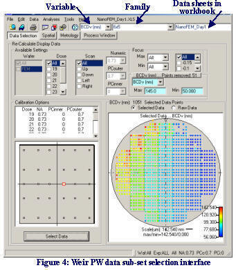
The Weir data workbook contains a primary data sheet as well as site and header information sheets for the layout. The workbook will also eventually contain analysis reports plus additional data sheets. The calculated Full-field focus will be stored in one of these datasheets and listed in the datasheet combo control located in the upper right of the interface shown in figure 4. To load a secondary datasheet, simply select it from this control. We will discuss this in more detail in the next section. Variable selection is simply a matter of choosing the variable from the drop-down combo.
Raw Metrology as well as Weir Workbook data can be directly imported into Weir PW. As in the "Weir Main" interface, the "File" menu provides access to the Weir Layout Library for one-click updates of the exposure layout when needed.
The controls at the top of this page provide automated data subset selection prior to analysis. In the instance shown in the figure the "BCDv" metrology variable is used to limit the acceptable range of analysis data by restricting "BCDv" variation to points that lie between 50 and 145 nm. This four-field control segment is located in the right-central portion of the interface shown. Pressing the command button, located immediately above the -culling-by-variable combo, will plot a histogram of the selected variable to assist in the proper selection of range limits.
Data points will be culled when the "Select Data" command button is pressed and the number of points removed will be displayed on the command button immediately above the drop-down variable combo. The command button, in this example, is also reporting that 51 data points were removed from the raw data using this control.
The mouse can also be used to provide an even simpler method of culling selected data points or field sites. Use the mouse to box-in and cull data points using either the wafer or field plots shown in figure 4. Selecting a field-site, from the left-side graphic, will remove all occurrences of the site from the data. Selecting data on the wafer plot will remove individual data points for selected or all wafers in the data. Data points are never actually "deleted" and can always be recovered using the mouse popup menu or by re-specifying the data selection in this interface.
Process Window Setup
To begin the
Dose-Response Analysis, select the Process Window tab and the interface shown in
figure 5 will appear. The thee images of the interface in figure 5 show only the
top-half of the screen. The output results and graphics as well as the analysis
calling-tabs are located below this region as shown in figure 6.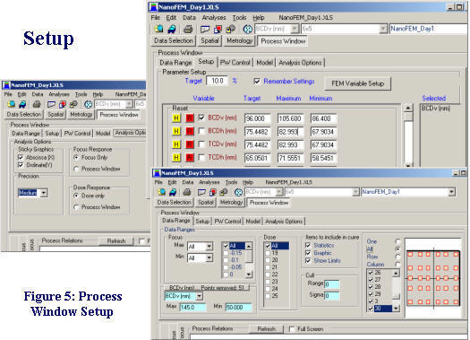
The Process Window (PW) interface has four setup tabs, the first of which provides additional data culling and site-selection as shown in the lower half of figure 5. The "Setup" tab provides the variable and control limit selection utilities (upper right of the figure).
Simply check a variable to include it in the analysis. Optionally press the yellow "H" command button to display a histogram of the variable. The "R" command will reset the control-limit parameters to those of the suggested variable statistics.
In this analysis the user has entered a 10% Exposure Latitude (EL) that will be calculated for the Maximum and Minimum control-limits of each variable. The target size for the BCDv variable has been set to 96 nm.
"Analysis
Options" are set using the 5th tab's interface shown in the left-side of the
figure. We will be conducting a "Dose" analysis to determine the Best
Dose, Exposure latitude, Focus, DoF and Feature uniformity each focus setting. A
"Medium" analysis precision has been selected and the curves will be fit to a
"Dose Polynomial" as shown by the selection of the "Dose Response" option button
control. Either the "Dose Polynomial" or "Process Window" algorithm can be
selected for this analysis.
As a final step in the setup, the field sites included in the data are shown on the right side of the "Data Selection" tab, shown in the lower right side of figure 5. This figure shows a selection with "All" sites selected for analysis and the corresponding field-layout graphic has all of it's sites highlighted.
To select individual sites, set the option button to "One", the site nearest the center of the field will be automatically selected, it's location on the graphic will be highlighted to the larger square shown here and it's site-number will be checked in the listing to the left of the graphic. An example where two sites have been selected is shown in figure 6. You can select additional sites either by checking the site number or by moving the mouse over the graphic until an "X" appears over the site. Click on the "X" to either select or de-select it from the list.
Running the Dose Uniformity Analysis
From the Data Selection interface, select the Process Window push-button to access the general analysis screen. Begin the Dose-Response analysis by pressing the "Dose" tab to the left and below this area of the interface; this area is shown in figure 6. The Weir PW software will automatically cycle through each selected site on the field and generate a complete set of Feature-size graphs as a function of dose for each site and tool-focus setting.
Theses graphs will most likely exhibit some non-linear response of the feature to dose variation since the contain the feature perturbations due to focus as well as dose. We will see how to remove these perturbations a little later in the discussion. First we should review the information and reports gained from this analysis.
Resulting Plots & Data
A typical "BCD v Dose" plot for five field sites is shown in figure 6 for the sites mapped in the field-schematic on the lower right of figure. While running the analysis, the spreadsheet will update analysis results with the three reports shown in Table #1, these reports are summarized on the "Index" spreadsheet located on the 2nd tab of the data workbook. To access any report simply click on the report hyperlink and the proper spreadsheet will be displayed
These reports are summarized in the table below and can also be viewed in the data's Weir Data Workbook.
|
Dose Report spreadsheets saved in the Weir Workbook |
|
| DoseResponseReport | Formal report summarizing the analysis. Includes setup, culling information and IsoFocal Dose for each site. The report also presents a statistical summary of the Best Dose, DoseRange, Best Focus, Focus Range and Dose Latitude for the reticle as for each site. |
| DoseResponse | Summary of the calibration offset, slope and residuals along with the target (best) dose and it's dose latitude. An entry is made for every feature, sit-location and focus value selected. |
| DoseUniformity |
A data sheet that can be analyzed and modeled in Weir PW for the Dose, Focus and Dose Latitude uniformity across the exposure field. One field is created containing all of the features measured (BCD, TCD etc) for the optimum focus and dose needed to achive the target feature size. The variation of full-profile feature response across experiment range and it's smaller process window can be directly analyzed. |
Dose Uniformity Analysis
To see the response
of this exposure tool to the reticle while trying to achive the desired target
size, next select the "DoseUniformity" data sheet from the data combo shown with
the red-ellipse around it in figure 7. Recall that this data set and spreadsheet
was
 created
when we ran the analysis displayed in figure 6.
created
when we ran the analysis displayed in figure 6.
In figure 7, we chose to model the response of each row of the scanner field using the "Row" Model selected from the "Model Components" tab of the Spatial Interface. This model will allow us to view the behavior of the dose as it varies across the lens slit of the scanner.
The Piston is the offset or optimum exposure-dose for the field. You can find the coefficients calculated for each row in the "FieldRowModel_BCDh_nm_Dose" spreadsheet that was just entered in the workbook. If you have multiple fields on the wafer/lot, each fields values are summarized on the "FieldModel_BCDh(nm)Dose[AllFields]" spreadsheet. Notice that each spreadsheet contains the name of the data variable selected for the analysis plus the type of analysis. Look in the "Index" spreadsheet for a hyperlink to each spreadsheet created.
Modeling Focus with the ASML and other Models of Weir PSFM
Return to the Weir Main interface and select the Weir PSFM Analysis Uniformity interface. The "RawFocus" datasheet will automatically load and any of four separate models can be applied to the focus variables.
The model shown here tells us that there is a significant mount of -23.8 urad tilt to each row of the field plus curvature in dose-response across the lens. The average of these values will tell us the response characteristics of the lens. The upper-left corner of the field also exhibits a large change in the required dosage to achieve the target size feature.
To help in understanding this response, we should examine the raw dose-uniformity data shown in figure 8.

Plot figure 8 by first turning of the spatial model by selecting the "No Modeling" option button. Next select the "Display Selection" tab and the "Vector" radio button. Plot the data by clicking on the "Field" tab once again. Now we can clearly see the dose uniformity from site-to-site. This is an excellent method for evaluating new reticles and designs since any errors in the design will quickly show up on the plot.
You can edit the
titles, lables, scale and other plot features by right-clicking on the plot. In
this figure we hae increased the size of the vector-sites by changing the "Size"
value to 8 on the graph-edit options interface shown in the lower right.
To view the raw dose uniformity as a function of the site's location within the slit box in the entire field with the left mouse-button. Next select the "Plot Selected Data/ XYplot by Column" menu item from the pop-up menu. A XY graph similar to that shown in figure 9 will be created.
To add the box-plots
to the graph again right-click on the graph and select the BoxPlot and
Contour Profiles check boxes as shown in the lower half of figure 9. The
"Color Profiles" selection will assign a scaled color value to each member of
the box-plot population with red being at the 50% population median and the
remaining colors scaling out to dark blue and finally black for out-of-control
points.
While the slit can be a strong contributor to dose non-uniformity, the actual exposure is set by the speed of the reticle scan. If there is any variation in speed across the field the effective exposure will vary. You can view the raw dose uniformity by selecting the "Plot Selected Data/ XYplot by Rows" menu item from the pop-up menu after once-again boxing in the entire vector fields as we did previously. An XY graph similar to that shown in figure 10 will plot the variation along the scan.
Figure 10 for this
tool shows about 2 mj/cm2 variation in dose along the scan. The variation is
sytematically changing andthe variation seen at +5 mm above field center may
signify a scan problem on the stage. The two out-of-control plots on the upper
left of the reticle can be seen on the 12mm x-axis plot. The uniformity
otherwise shown suggest that theses two sites are probably the result of the
reticle manufacturing process rather than the scanner.
It's not uncommon to see a systematic strong change in dose at the start or scan of the reticle. Vendors always want to maximize the number of wafers exposed with a tool. If the reticle stage begins it's directional reverse scan too soon or does not drop acceleration before exposure begins, the exposure seen by the reticle will change at the last (or first) few millimeters of the scan.
The Dose-Latitude % Uniformity across the exposure is easily plotting in the same manner as shown in figure 11.
First change the selected variable from "feature_Dose" to "feature_%Latitude" using the left-most combo at the top of the interface as shown in figure 7. Then plot the uniformity using the same tools as we did for the Dose Uniformity plots.
The plot of figure 7 highlights four sites that exhibit lower exposure latitude. This variation is probably due to OPC or proximity problems in the feature design.
Using this technique you can easily and quickly plot the sensitivity of the process to Focus Uniformity and the absolute Dose-Latitude.
Removing Exposure-Tool Influence: True Process Response to Dose
As we have seen the
exposure tool can be a significant contributor to effective-dose variations
across the field. Photoresist evaluations, simulator setup, anti-reflective
coating (ARC) evaluations and other film studies should try to minimize or
eliminate the tool from the analysis. This is not as simple as it would first
seem because the wavefront emanating from the exposure tool will not be uniform
in focus, reticles can bow or warp with heating and the very act of
clamping the reticle on the stage platen may introduce stress warping.
Since we know the feature response at every site across the field, our analysis can calculate the response without these errors to derive the true process or film response. This plot is easily derived for the user by simply selecting the "Dose @ Best Focus" analysis tab on the Weir PW interface as shown in figure 12.
The analysis shown in figure 12 addresses the true process response for two features (BCDv and BCDh). In this experiment the user has reduced the target feature size to 65 nm.
Figure 12 shows two very distinct and separate response curves families for these two features. Notice how the curvature and spread of the curves has been reduced for almost all of the sites. This represents the true process response for each site on the reticle.
A second set of curves, in red and blue, plots the Optimum Focus for each site as a function of the dose. These values are plotted against the right-hand ordinate of the graph. The optimum focus for each site should be flat and constant across the range of process dose response. A quality reticle will exhibit a minimum of focus variation across the field at best focus.
In the example of figure 12, we see the horizontal (red) and vertical (blue) feature response to focus quite differently for dose levels greater than 21 mj/cm2. This suggests that even though both features can be imaged at 65 nm, the process may not be controllable with exposures greater than 21 mj/cm2.
Dose @ Best Focus Reports & Graphs
During the Dose at Best Focus Analysis, Weir PW generates two reports that will be found on the following spreadsheets:
|
Dose @ Best Focus Report spreadsheets saved in the Weir Workbook |
|
| Dose_atBestFocusReport | Formal report summarizing the analysis. of the process dose response for two features across the exposure field. Includes setup, culling information and IsoFocal Dose for each site. The report also presents a statistical summary of the Best Dose, DoseRange, Best Focus, Focus Range, Depth of Focus, Exposure Latitude and Dose Latitude for the reticle and for each site. |
| DoseUniformity_atBF | Weir PW data sheet of the process response of the reticle without exposure tool de-focus perturbations. Includes the feature Dose Uniformity, EL%, Best Foucs, DoF and the uniformity of focus across the exposure tool when the feature is at the UCL and LCL limits. Each feature is treated as a separate wafer of data in this format. |
The
DoseUniformity_atBF spreadsheet is unique because it now plots the
uniformity of dose needed to achieve the target critical dimension without the
influence of defocus introduced by the exposure tool. This is
therefore the best estimate of the Reticle's feature response to dose.
Data now clearly shows the response of the reticle structures when trying to
achieve the target feature size.
Figure 13 provides graphs of the same data as figure 8 however the signature of the reticle is now clearly seen in the reduced dose range needed to achieve a 65 nm feature.
The
Focus uniformity plot for this form of the analysis is interesting
because the deFocus errors of the exposure tool have been removed. We are
therefore plotting an optimum focus response setting for each site on the
reticle that is a function of the curvature and symmetry of response of the site
to dose variation. Defocus is strictly a function of the structure and proximity
response of the reticle feature as constructed by the photomask manufacturer.
Figure 14 was created using the contour plot selection on the "Focus" variable for the "BCDh" and "BCDv" features from the "DoseUniformity_atBF" datasheet. In this case the variables (BCD h &v) were presented as separate "wafers" of data so the "Data Selection" tab was used to select only one wafer of data for each plot. The histograms to the left of the plot were created by boxing in the whole field of data with the left mouse-button and selecting Histogram plot form the pop-up menu.
Report Publishing to the WebDoseUniformity_atBF
Any of the Weir Reports are in Microsoft Excel spreadsheet format. This means you can publish modify, annotate and publish them to any web site by the the "File/SaveAs" menu command and selecting the "html" format. We can easily plot similar plots for the Focus, EL% and DoF variables.
Moving to Other Weir Interfaces
Weir program interfaces work interactively. You can move from Weir Main to any of the other five interfaces using the button-bar keys or the menu. Data is automatically transferred between interfaces. Any interface can load and, using the Weir Layout Library, configure exposure layouts for the arrays. Only the Weir Main interface can create Layout and Reticle Library Entries and Macros for the Weir Daily Monitor and DMA programs.
Interrupting Processing
-
The "ESC" key will interrupt any processing if it is held depressed.
-
Weir Reports can be saved to any website. To save the report, open it's spreadsheet in Excel and select the "File/SaveAs" menu. When the pop-up interface appears, select the "Web (htm,html)" format.
Graph Customization
-
Graphs are easily copied using the Edit Menu selections, the button bar and by boxing-in a section of any plot with the mouse.
-
To edit titles, rescale graphs, and add box-plots, trend-lines and fitted curves, right click on the graph and use the Graphic-Editor interface.
SpreadSheet Control
-
A "Spreadsheet" menu is located near the top right-hand corner of the Weir program interfaces. It will be listed as the name of the loaded Weir Workbook. The menu shown in figure 3 is using the name "KLA_SAMPLE.XLS".
-
Clicking on any spreadsheet menu will bring it to the forefront in the Excel Workbook.
-
Selecting the "Delete Worksheet" submenu will open an interface that will interactively allow multiple worksheets to be deleted from the workbook.
-
An "Index" worksheet positioned at the 3rd tab of the Weir Data workbook lists and links all of the worksheets created for data, reports and analysis summaries.
Automation
-
This entire analysis sequence can be automated to two-clicks of the mouse using Weir DM and Weir Automation Macros.
-
Weir DMA provides an external program portal for non-interactive analysis by Advance Process Control and Factory Automation programs.
TEA Systems
TEA Systems offers products to model films, photomasks, wafers, feature profiles, process and lens data for characterization and setup of semiconductor design, simulators, tools and the process.
TEA Systems, a privately held corporation since 1988, specializes in advanced, intelligent modeling of the semiconductor process and toolset. Products from TEA allow the user to decouple process, tool and random perturbations for enhanced process setup & control.
TEA Systems products include:
Weir PSFM: Full-wafer/field/scan analysis tool for FOCUS derived from proprietary defocus sensitive features.
Weir PW: Reticle/Full-wafer/field/scan analysis for any metrology with advanced process window capabilities for both wafer and photomask control.
LithoWorks PEB: A tool to link and correlate profile, film and critical element control to thermal reactions such as PEB and ChillPlate
Weir DMA: Macro Automation interface for Weir PSFM and Weir PW for external program calling, automated data gathering or one-button analysis of commonly used sequences. Includes data trending and web interface.
* An exposure cell, or Lithograph Cell, consists of the exposure tool (scanner) and it's associated wafer processing clean-tracs.
** Metrology Recipe: a program layout that d
References
[1] J. W. Bossung, “Projection Printing Characterization”, Developments in Semiconductor Microlithography II, Proc. of SPIE(1977) Vol. 100, pp. 80-84
[2] C. Ausschnitt, “Rapid Optimization of the lithographic process window”, SPIE vol 1088 (1989) pp. 115-123
[3] C.Mack, J. Byers, “Improved model for focus-exposure data analysis”, Proc of SPIE (2003) 5038-39, pp396-405* Excel is a trademark of Microsoft Corporation
* KLA is a tradename of KLA Instruments
* ASML is a tradename of ASM Lithography
ã Copyright 2006 TEA Systems Corporation, All rights reserved. Legal
TEA Systems
Corp. | Tel: +1 610 682 4146
65 Schlossburg St., Alburtis, PA USA